Tutorial 05: Kernels and averages

Simulating swarming models requires expensive mean-field convolution operations of the form:

\[J^i = \frac{1}{N}\sum_{j=1}^N K(|X^j-X^i|) U^j,\]

for \(1\leq i\leq N\), where \((X^i)_{1\leq i \leq N}\) are the positions of the particles, \((U^j)_{1\leq j\leq N}\) are given vectors and \(K\) is an observation kernel. Typically, \(K(|X^i-X^j|)\) is equal to 1 if \(X^i\) and \(X^j\) are at distance smaller than a fixed interaction distance and 0 otherwise. Other kernels are defined in the module sisyphe.kernels. Below, we show a simple application case.

Linear local averages

First, some standard imports…

import time
import math
import torch
from matplotlib import pyplot as plt

use_cuda = torch.cuda.is_available()
dtype = torch.cuda.FloatTensor if use_cuda else torch.FloatTensor

Let the \(N\) particles be uniformly scattered in a box of size \(L\) with interaction radius \(R\).

N = 100000
L = 1.
R = .15

pos = L*torch.rand((N,2)).type(dtype)

We can also assume that the particles have a bounded cone of vision around an axis (defined by a unit vector). The default behaviour is a full vision angle equal to \(2\pi\) in which case the axis is a None object. Here we take a cone of vision with angle \(\pi/2\) around an axis which is sampled uniformly. For the sisyphe.particles.KineticParticles, the default axis is the velocity.

angle = math.pi/2
axis = torch.randn(N,2).type(dtype)
axis = axis/torch.norm(axis,dim=1).reshape((N,1))

Let us create an instance of a particle system with these parameters.

from sisyphe.particles import Particles

particles = Particles(
    pos = pos,
    interaction_radius = R,
    box_size = L,
    vision_angle = angle,
    axis = axis)

Note

By default, the system and the operations below are defined with periodic boundary conditions.

As a simple application, we can compute the number of neighbours of each particle and print the number of neighbours of the first particle. This operation is already implemented in the method number_of_neighbours(). It simply corresponds to the average:

\[N^i_\mathrm{neigh} = \sum_{j=1}^N K(|X^j-X^i|).\]

Nneigh = particles.number_of_neighbours()

Nneigh0 = int(Nneigh[0].item())

print("The first particle sees " + str(Nneigh0) + " other particles.")

Out:

The first particle sees 1754 other particles.

For custom objects, the mean-field average can be computed using the method linear_local_average(). As an example, let us compute the center of mass of the neighbours of each particle. First we define the quantity \(U\) that we want to average. Here, since we are working on a torus, there are two: the sine and the cosine of the spatial coordinates.

cos_pos = torch.cos((2*math.pi / L) * particles.pos)
sin_pos = torch.sin((2*math.pi / L) * particles.pos)

Then we compute the two mean field averages, i.e. the standard convolution over the \(N\) particles. The center of mass along each dimension is the argument of the complex number whose coordinates are the average cosine and sine.

average_cos, average_sin = particles.linear_local_average(cos_pos, sin_pos)
center_x = torch.atan2(average_sin[:,0], average_cos[:,0])
center_x = (L / (2*math.pi)) * torch.remainder(center_x, 2*math.pi)
center_y = torch.atan2(average_sin[:,1], average_cos[:,1])
center_y = (L / (2*math.pi)) * torch.remainder(center_y, 2*math.pi)

center_of_mass = torch.cat((center_x.reshape((N,1)), center_y.reshape((N,1))),
                            dim=1)

Out:

[pyKeOps] Compiling libKeOpstorch3dcd0c2195 in /data/and18/.cache/pykeops-1.5-cpython-38:
       formula: Sum_Reduction(((Step((Var(5,1,2) - Sum(Square((((Var(0,2,1) - Var(1,2,0)) + (Step(((Minus(Var(2,2,2)) / Var(3,1,2)) - (Var(0,2,1) - Var(1,2,0)))) * Var(2,2,2))) - (Step(((Var(0,2,1) - Var(1,2,0)) - (Var(2,2,2) / Var(4,1,2)))) * Var(2,2,2))))))) * Step((Var(7,1,2) + (Sum(((((Var(0,2,1) - Var(1,2,0)) + (Step(((Minus(Var(2,2,2)) / Var(3,1,2)) - (Var(0,2,1) - Var(1,2,0)))) * Var(2,2,2))) - (Step(((Var(0,2,1) - Var(1,2,0)) - (Var(2,2,2) / Var(4,1,2)))) * Var(2,2,2))) * Var(6,2,0))) / Sqrt(Sum(Square((((Var(0,2,1) - Var(1,2,0)) + (Step(((Minus(Var(2,2,2)) / Var(3,1,2)) - (Var(0,2,1) - Var(1,2,0)))) * Var(2,2,2))) - (Step(((Var(0,2,1) - Var(1,2,0)) - (Var(2,2,2) / Var(4,1,2)))) * Var(2,2,2)))))))))) * Var(8,4,1)),0)
       aliases: Var(0,2,1); Var(1,2,0); Var(2,2,2); Var(3,1,2); Var(4,1,2); Var(5,1,2); Var(6,2,0); Var(7,1,2); Var(8,4,1);
       dtype  : float32
...
Done.

In the method linear_local_average(), the default observation kernel is a LazyTensor of size \((N,N)\) whose \((i,j)\) component is equal to 1 when particle \(j\) belongs to the cone of vision of particle \(i\) and 0 otherwise. To retrieve the indexes of the particles which belong to the cone of vision of the first particle, we can use the K-nearest-neighbours reduction provided by the KeOps library.

from sisyphe.kernels import lazy_interaction_kernel

interaction_kernel = lazy_interaction_kernel(
    particles.pos,
    particles.pos,
    particles.R,
    particles.L,
    boundary_conditions = particles.bc,
    vision_angle = particles.angle,
    axis = particles.axis)

K_ij = 1. - interaction_kernel

neigh0 = K_ij.argKmin(Nneigh0, dim=1)[0]

print("The indexes of the neighbours of the first particles are: ")
print(neigh0)

Out:

[pyKeOps] Compiling libKeOpstorchaf7a666555 in /data/and18/.cache/pykeops-1.5-cpython-38:
       formula: ArgKMin_Reduction((Var(8,1,2) - (Step((Var(5,1,2) - Sum(Square((((Var(0,2,1) - Var(1,2,0)) + (Step(((Minus(Var(2,2,2)) / Var(3,1,2)) - (Var(0,2,1) - Var(1,2,0)))) * Var(2,2,2))) - (Step(((Var(0,2,1) - Var(1,2,0)) - (Var(2,2,2) / Var(4,1,2)))) * Var(2,2,2))))))) * Step((Var(7,1,2) + (Sum(((((Var(0,2,1) - Var(1,2,0)) + (Step(((Minus(Var(2,2,2)) / Var(3,1,2)) - (Var(0,2,1) - Var(1,2,0)))) * Var(2,2,2))) - (Step(((Var(0,2,1) - Var(1,2,0)) - (Var(2,2,2) / Var(4,1,2)))) * Var(2,2,2))) * Var(6,2,0))) / Sqrt(Sum(Square((((Var(0,2,1) - Var(1,2,0)) + (Step(((Minus(Var(2,2,2)) / Var(3,1,2)) - (Var(0,2,1) - Var(1,2,0)))) * Var(2,2,2))) - (Step(((Var(0,2,1) - Var(1,2,0)) - (Var(2,2,2) / Var(4,1,2)))) * Var(2,2,2))))))))))),1754,0)
       aliases: Var(0,2,1); Var(1,2,0); Var(2,2,2); Var(3,1,2); Var(4,1,2); Var(5,1,2); Var(6,2,0); Var(7,1,2); Var(8,1,2);
       dtype  : float32
...
Done.
The indexes of the neighbours of the first particles are:
tensor([    0,    29,   130,  ..., 99811, 99868, 99982], device='cuda:0')

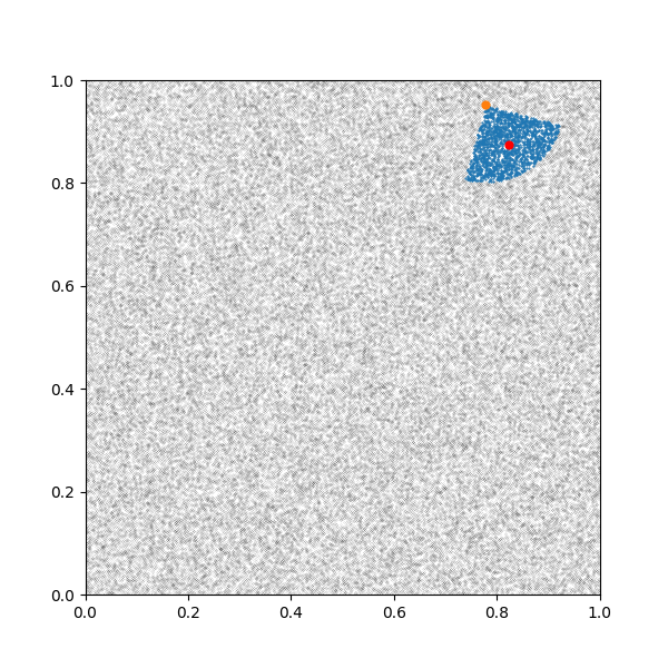
Finally, a fancy display of what we have computed. We plot the full particle system in black, the first particle in orange, its neighbours in blue and the center of mass of the neighbours in red.

xall = particles.pos[:,0].cpu().numpy()
yall = particles.pos[:,1].cpu().numpy()

x = particles.pos[neigh0,0].cpu().numpy()
y = particles.pos[neigh0,1].cpu().numpy()

x0 = particles.pos[0,0].item()
y0 = particles.pos[0,1].item()

xc = center_of_mass[0,0].item()
yc = center_of_mass[0,1].item()


fig, ax = plt.subplots(figsize=(6,6))
ax.scatter(xall, yall, s=.003, c='black')
ax.scatter(x, y, s=.3)
ax.scatter(x0, y0, s=24)
ax.scatter(xc, yc, s=24, c='red')
ax.axis([0, L, 0, L])
ax.set_aspect("equal")

Nonlinear averages

In some cases, we need to compute a nonlinear average of the form

\[J^i = \frac{1}{N}\sum_{j=1}^N K(|X^j-X^i|) b(U^i,V^j),\]

where \((U^i)_{1\leq i \leq N}\) and \((V^j)_{1\leq j \leq N}\) are given vectors and \(b\) is a given function. When the binary formula \(b\) can be written as a LazyTensor, this can be computed with the method nonlinear_local_average().

For instance, let us compute the local mean square distance:

\[J^i = \frac{\sum_{j=1}^N K(|X^j-X^i|) |X^j-X^i|^2}{\sum_{j=1}^N K(|X^j-X^i|)}.\]

In this case, we can use the function sisyphe.kernels.lazy_xy_matrix() to define a custom binary formula. Given two vectors \(X=(X^i)_{1\leq i\leq M}\) and \(Y = (Y^j)_{1\leq j\leq N}\), respectively of sizes \((M,d)\) and \((N,d)\), the \(XY\) matrix is a \((M,N,d)\) LazyTensor whose \((i,j,:)\) component is the vector \(Y^j-X^i\).

from sisyphe.kernels import lazy_xy_matrix

def b(x,y):
    K_ij = lazy_xy_matrix(x,y,particles.L)
    return (K_ij ** 2).sum(-1)

x = particles.pos
y = particles.pos
mean_square_dist = N/Nneigh.reshape((N,1)) * particles.nonlinear_local_average(b,x,y)

Since the particles are uniformly scattered in the box, the theoretical value is

\[MSD_0 = \frac{\int_0^R \int_0^{\pi/2} r^3 \mathrm{d}r\mathrm{d}\theta}{\int_0^R \int_0^{\pi/2} r \mathrm{d}r\mathrm{d}\theta} = \frac{R^2}{2}\]

print("Theoretical value: " + str(R**2/2))
print("Experimental value: " + str(mean_square_dist[0].item()))

Out:

Theoretical value: 0.01125
Experimental value: 0.01103969756513834