Note
Click here to download the full example code
Mills
Examples of milling behaviours.
First of all, some standard imports.
import os
import sys
import time
import math
import torch
import numpy as np
from matplotlib import pyplot as plt
import sisyphe.models as models
from sisyphe.display import display_kinetic_particles

use_cuda = torch.cuda.is_available()
dtype = torch.cuda.FloatTensor if use_cuda else torch.FloatTensor
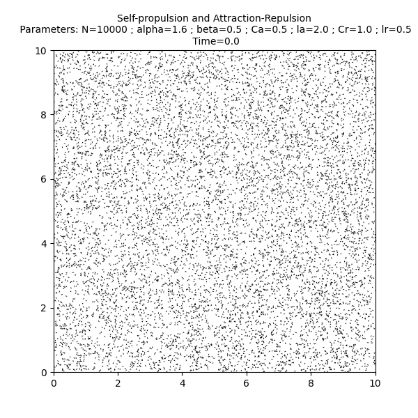
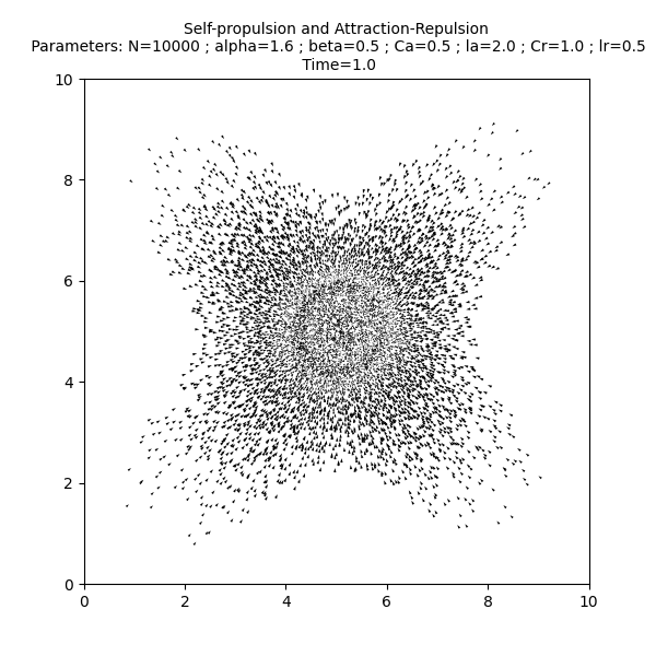
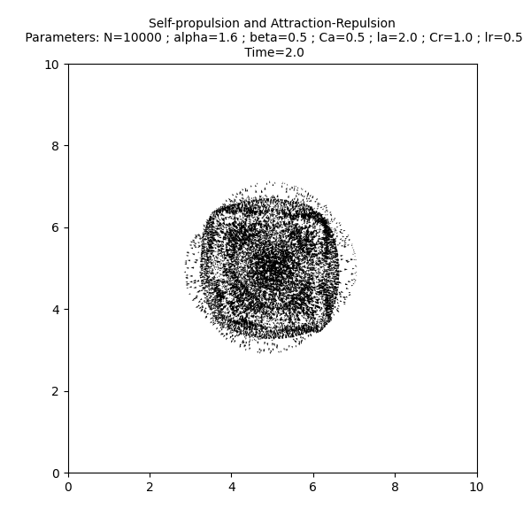
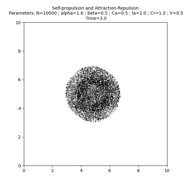
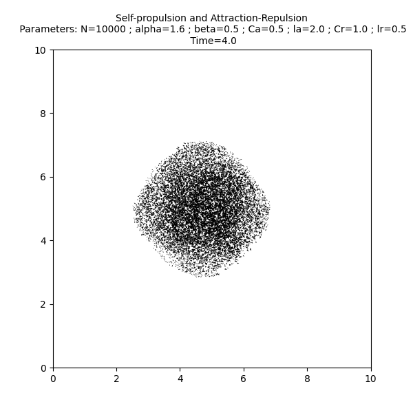
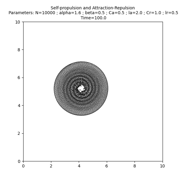
Milling in the D’Orsogna et al. model
Let us create an instance of the attraction-repulsion model introduced in
D’Orsogna, Y. L. Chuang, A. L. Bertozzi, L. S. Chayes, Self-Propelled Particles with Soft-Core Interactions: Patterns, Stability, and Collapse, Phys. Rev. Lett., Vol. 96, No. 10 (2006).
The particle system satisfies the ODE:
where \(U\) is the Morse potential
N = 10000
mass = 1000.
L = 10.

Ca = .5
la = 2.
Cr = 1.
lr = .5

alpha = 1.6
beta = .5
v0 = math.sqrt(alpha/beta)

pos = L*torch.rand((N,2)).type(dtype)
vel = torch.randn(N,2).type(dtype)
vel = vel/torch.norm(vel,dim=1).reshape((N,1))
vel = v0*vel

dt = .01

simu = models.AttractionRepulsion(pos=pos,
                 vel=vel,
                 interaction_radius=math.sqrt(mass),
                 box_size=L,
                 propulsion = alpha,
                 friction = beta,
                 Ca = Ca,
                 la = la,
                 Cr = Cr,
                 lr = lr,
                 dt=dt,
                 p=1,
                 isaverage=True)
Run the simulation over 100 units of time and plot 10 frames. The ODE system is solved using the Runge-Kutta 4 numerical scheme.
frames = [0,1,2,3,4,5,10,40,70,100]

s = time.time()
it, op = display_kinetic_particles(simu,frames)
e = time.time()

Out:
Progress:0%
Progress:1%
Progress:2%
Progress:3%
Progress:4%
Progress:5%
Progress:6%
Progress:7%
Progress:8%
Progress:9%
Progress:10%
Progress:11%
Progress:12%
Progress:13%
Progress:14%
Progress:15%
Progress:16%
Progress:17%
Progress:18%
Progress:19%
Progress:20%
Progress:21%
Progress:22%
Progress:23%
Progress:24%
Progress:25%
Progress:26%
Progress:27%
Progress:28%
Progress:29%
Progress:30%
Progress:31%
Progress:32%
Progress:33%
Progress:34%
Progress:35%
Progress:36%
Progress:37%
Progress:38%
Progress:39%
Progress:40%
Progress:41%
Progress:42%
Progress:43%
Progress:44%
Progress:45%
Progress:46%
Progress:47%
Progress:48%
Progress:49%
Progress:50%
Progress:51%
Progress:52%
Progress:53%
Progress:54%
Progress:55%
Progress:56%
Progress:57%
Progress:58%
Progress:59%
Progress:60%
Progress:61%
Progress:62%
Progress:63%
Progress:64%
Progress:65%
Progress:66%
Progress:67%
Progress:68%
Progress:69%
Progress:70%
Progress:71%
Progress:72%
Progress:73%
Progress:74%
Progress:75%
Progress:76%
Progress:77%
Progress:78%
Progress:79%
Progress:80%
Progress:81%
Progress:82%
Progress:83%
Progress:84%
Progress:85%
Progress:86%
Progress:87%
Progress:88%
Progress:89%
Progress:90%
Progress:91%
Progress:92%
Progress:93%
Progress:94%
Progress:95%
Progress:96%
Progress:97%
Progress:98%
Progress:99%
Print the total simulation time and the average time per iteration.
print('Total time: '+str(e-s)+' seconds')
print('Average time per iteration: '+str((e-s)/simu.iteration)+' seconds')
Out:
Total time: 86.00608777999878 seconds
Average time per iteration: 0.008600608777999877 seconds
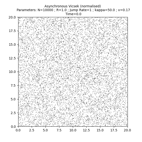
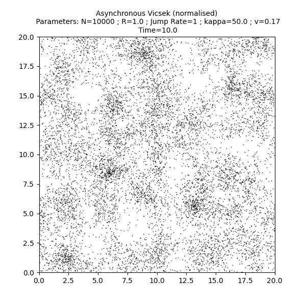
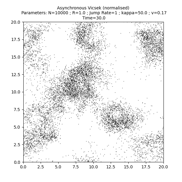
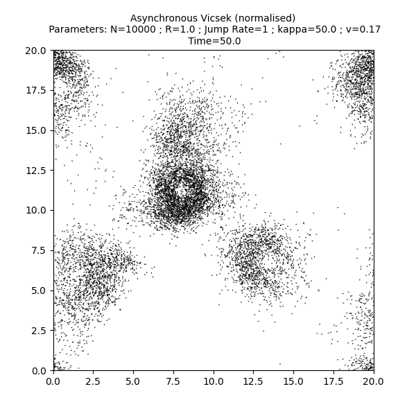
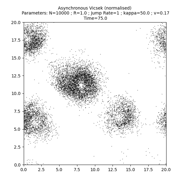
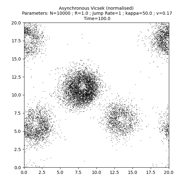
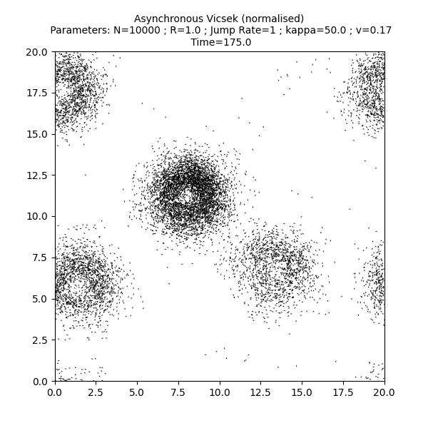
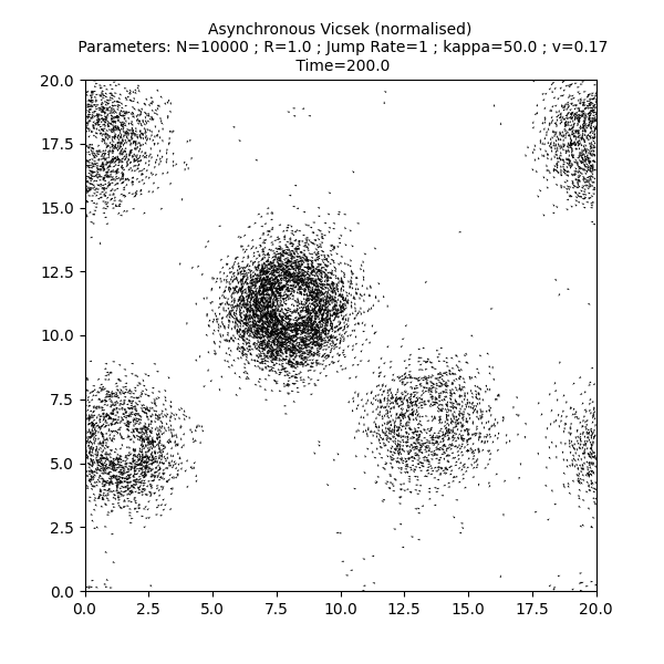
Milling in the Vicsek model
Let us create an instance of the Asynchronuos Vicsek model with a bounded cone of vision and a bounded angular velocity, as introduced in:
Costanzo, C. K. Hemelrijk, Spontaneous emergence of milling (vortex state) in a Vicsek-like model, J. Phys. D: Appl. Phys., 51, 134004
N = 10000
R = 1.
L = 20.

nu = 1
sigma = .02
kappa = nu/sigma

c = .175
angvel_max = .175/nu

pos = L*torch.rand((N,2)).type(dtype)
vel = torch.randn(N,2).type(dtype)
vel = vel/torch.norm(vel,dim=1).reshape((N,1))

dt = .01
We add an option to the target
target = {"name" : "normalised", "parameters" : {}}
option = {"bounded_angular_velocity" : {"angvel_max" : angvel_max, "dt" : 1./nu}}

simu=models.AsynchronousVicsek(pos=pos,vel=vel,
                 v=c,
                 jump_rate=nu,kappa=kappa,
                 interaction_radius=R,
                 box_size=L,
                 vision_angle=math.pi, axis = None,
                 boundary_conditions='periodic',
                 variant=target,
                 options=option,
                 sampling_method='projected_normal')
Run the simulation over 200 units of time and plot 10 frames.
# sphinx_gallery_thumbnail_number = -1

frames = [0, 10, 30, 50, 75, 100, 125, 150, 175, 200]

s = time.time()
it, op = display_kinetic_particles(simu,frames)
e = time.time()


Out:
Progress:0%
Progress:1%
Progress:2%
Progress:3%
Progress:4%
Progress:5%
Progress:6%
Progress:7%
Progress:8%
Progress:9%
Progress:10%
Progress:11%
Progress:12%
Progress:13%
Progress:14%
Progress:15%
Progress:16%
Progress:17%
Progress:18%
Progress:19%
Progress:20%
Progress:21%
Progress:22%
Progress:23%
Progress:24%
Progress:25%
Progress:26%
Progress:27%
Progress:28%
Progress:29%
Progress:30%
Progress:31%
Progress:32%
Progress:33%
Progress:34%
Progress:35%
Progress:36%
Progress:37%
Progress:38%
Progress:39%
Progress:40%
Progress:41%
Progress:42%
Progress:43%
Progress:44%
Progress:45%
Progress:46%
Progress:47%
Progress:48%
Progress:49%
Progress:50%
Progress:51%
Progress:52%
Progress:53%
Progress:54%
Progress:55%
Progress:56%
Progress:57%
Progress:58%
Progress:59%
Progress:60%
Progress:61%
Progress:62%
Progress:63%
Progress:64%
Progress:65%
Progress:66%
Progress:67%
Progress:68%
Progress:69%
Progress:70%
Progress:71%
Progress:72%
Progress:73%
Progress:74%
Progress:75%
Progress:76%
Progress:77%
Progress:78%
Progress:79%
Progress:80%
Progress:81%
Progress:82%
Progress:83%
Progress:84%
Progress:85%
Progress:86%
Progress:87%
Progress:88%
Progress:89%
Progress:90%
Progress:91%
Progress:92%
Progress:93%
Progress:94%
Progress:95%
Progress:96%
Progress:97%
Progress:98%
Progress:99%
Print the total simulation time and the average time per iteration.
print('Total time: '+str(e-s)+' seconds')
print('Average time per iteration: '+str((e-s)/simu.iteration)+' seconds')
Out:
Total time: 69.85851073265076 seconds
Average time per iteration: 0.003492925536632538 seconds
Total running time of the script: ( 2 minutes 38.151 seconds)